How Things Were · 1930
1930: Prices fall while jobs become harder to find
A redesigned Model A arrives as the downturn spreads from financial markets into daily household life.
In 1930, lower prices began to accompany a much harder employment picture. Economists and business leaders still hoped for recovery, but bank failures late in the year intensified uncertainty. Families did not experience the change equally: a secure paycheck could stretch farther at the grocery counter, while reduced hours or unemployment could erase that benefit. The year also produced a census that gives a detailed picture of the people, homes and occupations of the Model A era.
What everyday things cost
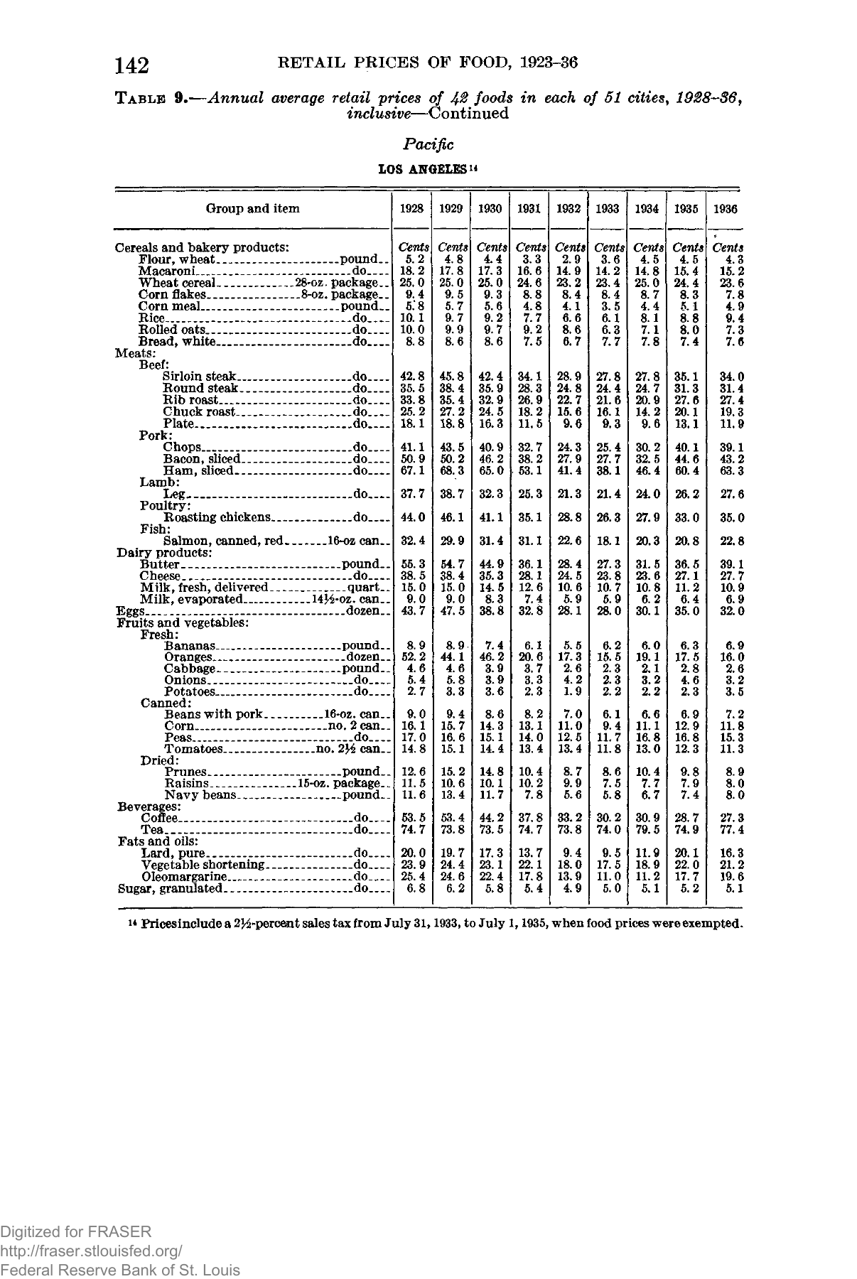
These are original dollars. Grocery prices below are annual Los Angeles averages, not national prices or a single store’s special. Bread is priced by the pound: the loaf example is a one-pound white loaf. Milk is delivered fresh milk sold by the quart.
| Grocery item and unit | 1930 Los Angeles price |
|---|---|
| Bread, white — one-pound loaf | 8.6¢ |
| Fresh milk, delivered — quart | 14.5¢ |
| Milk — gallon equivalent (4 quarts) | 58¢, calculated |
| Eggs — dozen | 38.8¢ |
| Butter — pound | 44.9¢ |
| Coffee — pound | 44.2¢ |
| Sugar — pound | 5.8¢ |
| Potatoes — pound | 3.6¢ |
| Sirloin steak — pound | 42.4¢ |
| Bacon, sliced — pound | 46.2¢ |
| Oranges — dozen | 46.2¢ |
Sources: BLS, Retail Prices of Food, 1923–36, Table 9, p. 142
Gasoline and the cost of using a Ford
| Gasoline, U.S. gallon | 1930 city-series average |
|---|---|
| Before state/federal tax | 16.16¢ |
| State/federal tax component | 3.79¢ |
| Price including those taxes | 19.95¢ |
This historical series covers 50 representative cities and averages first-of-month quotations. Local taxes are excluded. It is a comparison series, not the pump price at every station. Fuel grade, place and price competition could produce a different local amount.
A ten-gallon purchase at that tax-inclusive average would cost about $1.99. This is a calculation from the series, not an advertised fill-up. A driver also needed oil, tires, maintenance and registration; the fuel bill alone did not describe the full cost of ownership.
Sources: Hillary J. Fisher, MIT thesis (1938), Appendix A, Table XI; Automobile Facts and Figures (1937)
A movie ticket
| Documented example | Admission |
|---|---|
| 1930 local theater example | 40¢ adult; 25¢ student; 10¢ child, Auburn opening |
At the State Theatre’s opening in Auburn, California, on December 26, 1930, advertised admission was 40 cents for adults, 25 cents for students and 10 cents for children; loge seats cost 50 cents. This is a documented California opening-night price scale, not the average ticket nationwide. Seating location and customer category affected the cost, just as they do today.
Sources: City of Auburn: State Theatre opening, December 26, 1930
Buying a new Model A Ford
| Body style | Advertised base price, FOB Detroit |
|---|---|
| Standard Roadster | $450 |
| De Luxe Roadster | $520 |
| Phaeton | $440 |
| De Luxe Phaeton | $625 |
| Standard Coupe | $495 |
| De Luxe Coupe | $545 |
| Tudor Sedan | $495 |
| Fordor Sedan | $600 |
| Town Sedan | $640 |
| Victoria | $580 |
| Station Wagon | $640 |
These prices exclude accessories, transportation to the buyer’s locality and dealer additions. They are historical list-price examples, not guarantees of an unchanged price throughout the year. A used Ford might cost less, while financing added obligations. Some commercial body prices are not available in the cited list; no guessed pickup or AA truck price has been substituted.
Sources: Model A Ford Club of America: Prices When the Model A Was New
Ford refreshed the Model A’s styling for 1930, with a longer hood, sweeping fenders, a revised radiator treatment and smaller wheels. De Luxe models broadened the range. The Henry Ford reports nearly 1.16 million Model As sold in 1930, but notes that only a small share were open phaetons: many buyers preferred closed bodies with permanent roofs and roll-up windows. New styles could attract buyers, yet they could not fully offset the loss of purchasing power.
Sources: The Henry Ford: Henry Ford, Post-Model T
Putting the price in household terms
A $495 Tudor was a major durable purchase, unlike a few cents spent on bread. The buyer had to consider the down payment, future installments, running costs and the chance of keeping a job. Even a price that looked modest beside a house could represent months of saving. Price tags alone do not tell us who could afford the car.
The differences between bodies mattered in daily use. A closed sedan could serve a family in bad weather; an open roadster traded some protection and passenger space for a different experience. Delivery and truck bodies put the same broad Ford family into business use. See the club’s Model A Body Styles page for pictures and descriptions of passenger and commercial vehicles.
Homes, rent and the cost of a place to live
The 1930 census reported a median value of $4,778 for owned nonfarm homes and median monthly rent of $27.16 for rented nonfarm homes. These are different measurements: a reported property value is not a transaction price, and monthly rent is not a mortgage payment. Farms are excluded from these figures. The price of an individual house depended on its city, lot, size, condition and services, so neither figure describes every American’s housing.
Sources: 1930 Census, Population Vol. VI, Table 5, p. 7 · Sears Archives: home models and price ranges, 1927–1932
A catalog house package should not be compared directly with a finished house on its own lot. Freight, excavation, foundations, assembly, plumbing, wiring and local labor could change the total substantially. Renters faced a different budget: the monthly payment, heat and utilities, rather than the entire value of a building. Neighborhood and the condition of the property mattered as much as its floor plan.
Housing reference: the $4,778 figure on these pages is explicitly the 1930 census median reported value of owned nonfarm homes. It is not a measured annual national sale price for 1928, 1929 or 1931. The catalog ranges cover 1927–1932 and likewise should not be read as exact quotes for every model in every year.
What people did for a living
The historical employment series estimates 45.48 million employed people and 4.34 million unemployed in 1930, an 8.7 percent unemployment rate. Agricultural employment was about 10.34 million. These later-reconstructed annual estimates are useful for comparison, but they are not results from today’s monthly household survey, which did not yet exist. A worker still counted as employed could also face fewer paid hours.
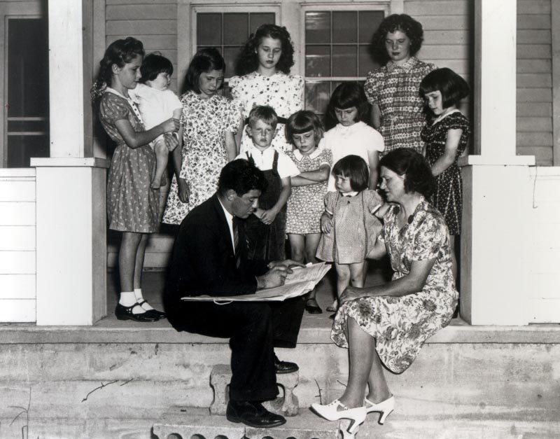
The occupation census records the breadth of working America: agriculture, manufacturing and mechanical industries, extraction of minerals, transportation and communication, trade, professional services, domestic and personal service, and clerical work. Nurses and teachers, merchants and bookkeepers, railroad engineers and mechanics all belonged to this economy. Women’s unpaid household labor was not represented like a wage-paying occupation, and discrimination restricted many workers’ choices.
Sources: 1930 Census: General Report on Occupations · Census historical employment table HS-29 · BLS: how Depression-era unemployment estimates were developed
| Work setting | Examples of period jobs |
|---|---|
| Farms and food | Farmers, hired hands, dairy workers, packers and grocers |
| Industry and building | Assembly workers, machinists, miners, carpenters and electricians |
| Transport and communications | Railroad crews, truck drivers, delivery workers and telephone operators |
| Stores and offices | Sales clerks, bookkeepers, typists and stenographers |
| Homes and public services | Domestic workers, cooks, teachers and nurses |
The economy and the Model A’s place in it
By November, regional banking crises helped turn hopes of an ordinary recovery into a deeper contraction. Depositors feared losing their savings; banks faced withdrawals and became less able to lend. A car buyer needed both confidence in future wages and access to cash or credit. The June 17 Smoot-Hawley tariff raised trade barriers and drew retaliation, adding difficulties to an already weakened world economy. It was a contributing policy problem, not the sole cause of the Depression.
Sources: Federal Reserve History: Banking Panics of 1930–31 · U.S. Senate: the Smoot-Hawley tariff
Why cheaper goods did not always mean easier living
For a household with reliable wages, a fall in retail prices could increase what its money bought. For a household facing reduced hours, unemployment or lost savings, the lower price could still be out of reach. Deflation could also make an unchanged debt more burdensome relative to earnings. This explains why later Model A advertising and price changes cannot be judged only by the number printed beside a body style.
Crime, law and public life
On June 11, 1930, Congress authorized the Bureau of Investigation’s national collection and compilation of uniform crime statistics. The program had previously been handled by the International Association of Chiefs of Police. Early reporting depended on participating police agencies; it was not an immediate complete count of every offense in the country. This limits claims that all crime suddenly rose by a precise nationwide percentage. Prohibition offenses, robberies, burglary and local violence remained concerns, but reliable interpretation requires attention to what the reports actually covered.
Sources: FBI historical timeline: national crime reporting in 1930
Crime stories were prominent in the press, but a notorious case is not a statistical measure of ordinary life in every town. Organized crime, property crime, corruption and racial violence need separate attention. Nor should hardship be treated as proof that unemployed people were criminals. The early national reporting system’s limits make sweeping year-to-year claims particularly risky.
Sources: FBI historical timeline: national crime reporting in 1930
Facts and dates from the year
- June 17: President Herbert Hoover signed the Smoot-Hawley tariff. Trading partners retaliated, worsening international trade conditions.
- April 1: census day; the population count was 122,775,046.
- June 11: national uniform crime-statistics collection was authorized for the Bureau of Investigation.
- November: regional bank panics intensified the downturn.
- Annual unemployment estimate: 8.7 percent.
Sources: U.S. Senate: the Smoot-Hawley tariff · FBI historical timeline: national crime reporting in 1930 · Census historical employment table HS-29
A look at the original grocery record